I'm currently working with a Sanger-generated 10-gene dataset, which includes a few fast-evolving genes. During the initial data exploration phase I used saturation plots to check for potential decay of phylogenetic signal caused by multiple substitutions (saturated nucleotide variation).
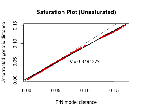
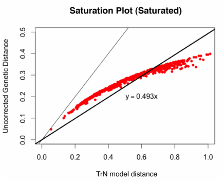
There are a lot of ways to visualize saturation. One method, which I believe was originally used by Philippe et al. (1994), is to plot the raw or uncorrected pairwise genetic distances in an alignment against model-corrected genetic distances. If the relationship is approximately linear, then the gene is not saturated; if the line curves or plateaus, there is evidence of saturation.
Here is an example of an unsaturated gene:
And an example of a saturated gene:
This is a really rough method, which should probably only be used as a preliminary exploration of your data. As far as I know, there is not an established slope value that says definitively, "yes, this gene is saturated." However, I do think it's a useful thing to look at, and it's really easy to do in R. You may want to look into APE's dist.dna command for all of the available models. Here is the R-code I used to make these simple plots:
library(ape)
###Input data: a phylip-format alignment file, converted to a 'DNAbin' object###
dat<-read.dna(file="myData.phy", format = "sequential", as.character=TRUE, skip=0)
dat<-as.DNAbin(dat)
###Convert to genetic distances###
dist<-dist.dna(dat, model="raw")
dist.corrected<-dist.dna(dat, model="TN93")
###Make plot###
plot(dist~dist.corrected, pch=20, col="red", xlab="TrN model distance", ylab="Uncorrected genetic distance", main="Saturation Plot")
abline(0,1, lty=2)
abline(lm(dist~dist.corrected), lwd=3)
lm_coef<-coef(lm(dist~dist.corrected))
text(0.1,0.05,bquote(y == .(lm_coef[2])*x))


 RSS Feed
