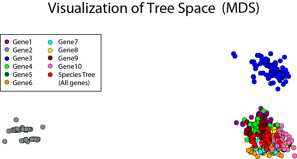
Here's a quick way to use R to visualize treespace! It's not necessarily the most rigorous analysis, but I think it's a useful tool for visualizing what's going on between your gene and species trees after an analysis like *BEAST.
Basically I'm computing a matrix of Robinson-Foulds (RF) distances between the trees produced in *BEAST, then plotting these using a Principal Coordinates Analysis (pcoa). Apparently the same analysis can also be implemented in the package TreeSetViz within Mesquite, although I wasn't able to get that to work :(
I found the tree.dist.matrix function on Dan Warren's github page. Thanks, Dan! Here's the rest of the code I used:
###
library(ape)
library(phangorn)
# import a single nexus file with all of the trees you want to plot. In order to make the colors
# work, each tree name should start with "geneName" and an underscore. Here's an example.
All.trees<-read.nexus(file="/Users/kathryneverson/Desktop/RTreeSpace.trees")
tree.dist.matrix <- function(trees, treenames=names(trees)){
N <- length(trees)
if(N != length(treenames)){
stop("Names and tree list must be the same length")
}
#Create an empty matrix for results
RF <- matrix(0, N, N)
for(i in 1:(N-1)){
#print(paste("Tree", i, "of", N))
for(j in (i+1):N){
RFd <- RF.dist(trees[[i]],trees[[j]])
if(RFd==0) RFd = 0.000000001
RF[i,j]<-RF[j,i]<-RFd
}
}
#Row and column names
rownames(RF) <- treenames
colnames(RF) <- treenames
RF
}
All.dist<-tree.dist.matrix(All.trees)
gene <- factor(gsub("_.*", "", rownames(All.dist), perl=TRUE))
levels(gene)
#there should be as many colors in this list as there are genes
cols = c('darkmagenta', 'azure4', 'blue', 'green', 'darkgreen', 'orange2', 'cyan', 'yellow2', 'red', 'black', 'darkred', 'hotpink')[gene]
All.pcoa<-pcoa(All.dist)
biplot(All.pcoa)
plot(All.pcoa$vectors[,1], All.pcoa$vectors[,2], type = "p", xlab = "", ylab = "",
pch=20, axes = FALSE, main = "Visualization of Tree Space (MDS)", col=cols)
legend('top', legend=levels(gene), cex = 0.5, pch = 20, col =c('darkmagenta', 'azure4', 'blue', 'green', 'darkgreen', 'orange2', 'cyan', 'yellow2', 'red', 'black', 'darkred', 'hotpink'))
###
NOTE: Calculating the RF distances is pretty slow, and I would not recommend trying to include thousands of trees. Here I thinned out my *BEAST tree files and just plotted 100 trees for each gene + the species tree.


 RSS Feed
